About Me

Agenda

1. Nutrifood's distribution problem — why it became a priority project

2. Data preparation & clustering — cleaning the mess before the math

3. Dynamic Spiral Optimization — from concept to production

4. Results and lessons learned — what worked, what hurt

5. Q&A session — as needed at the end, ask me anything

Nutrifood at a Glance

• Since 1979 — a pioneer of healthy FMCG in Indonesia, almost 50 years old
• Wide product portfolio:
  NutriSari — fruit drinks L-Men — high protein HiLo — high calcium Tropicana Slim — low calorie Lokalate — coffee W'dank — traditional drinks
• Reach: national — from Sabang to Merauke
• Scale: hundreds of SKUs, hundreds of distributors, sub-distributors, and retailers

A business this big has a distribution problem that is not simple at all.

How Nutrifood Distributes: Direct Shipment

The Math Behind It: Vehicle Routing Problem

Why Is This Hard?

A "simple" day looks like this:

• Purchase orders (PO) from 100 customers in one day
• One PO = one customer, but can contain many products with different volumes (m³) and weights (kg)
• Each PO tells us: total cubic & tonnage to send, and a date range for delivery
• One PO cannot be split into several shipments
• Each customer is served by Ciawi or Cibitung — never both

The number of possible route combinations explodes. No human — and no brute-force computer — can check them all. We need a smart approach.

Choosing the Algorithm: Why DSO?

How DSO Works — In Plain Words

DSO in Motion

The Algorithm Workflow

INPUT
  m >= 2   # number of points
  theta    # rotation angle (0..2π)
  r        # contraction rate
  k_max    # max iterations

PROCESS
  1  generate m random points x_i
  2  set k = 0
  3  find x* that gives min f(x*)
  4  rotate + contract every x_i
       with x* as the center
       k = k + 1
  5  repeat steps 3 and 4
  6  stop when k = k_max
       → output x*

The Core Mathematics

The transporter problem is a Mixed Integer Linear Programming (MILP) problem:

To solve it with DSO, we fold the constraints into one penalized objective:

where α, β are penalty constants that can be made very large. Break a rule → pay a huge penalty.

The One Tricky Part: Rotation in n Dimensions

DSO is easy to code in any language — except for one stone in your shoe: defining the rotation matrix for an n-dimensional problem.

• The rotation matrix is a product of many plane rotations (cross product of matrices)
• Why rotation? Rotation does not change the norm of a vector — agents move around the center without "jumping" distances

The Data: Customer Orders

One row = one sales order. A customer can have many orders per day. Each order has volume, weight, and a delivery-date window.

Notice customer 1004: one order of 12 m³ / 1.8 tons next to tiny orders of 0.04 m³ — the size range is huge.

The Data: Customer Details

The Data: Warehouses

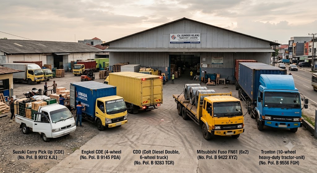
The Data: Vehicle Fleet

Nine vehicle types: from a small Carry (5 m³, cheap, can visit 7 stops) up to a 40-ft container (65 m³, expensive, only 2 stops). Bigger is not always better — cost per km grows fast.

What We Want the Algorithm to Produce

Take the order table… and let the algorithm fill three new columns for every sales order:

First Attempt: Brute Elegance

In the first iteration, I let DSO generate the delivery date and the vehicle grouping directly as candidate solutions. The stop order became part of the cost inside the objective function.

The reality check:

• DSO works in a continuous space (fractions), but our solutions are discrete (dates, truck IDs)
• The matrix dimension was huge — the rotation step ate an enormous amount of computation
• Finding a solution took very long, and the result was not optimal

First Attempt: The Result Was Far From Optimal

• Because the delivery date and vehicle grouping were generated directly by DSO…
• …the computer needed a very long time just to reach an acceptable solution — and even that was still far from optimal
• The reason: the problem dimension explodes — it depends on how many POs come in that day

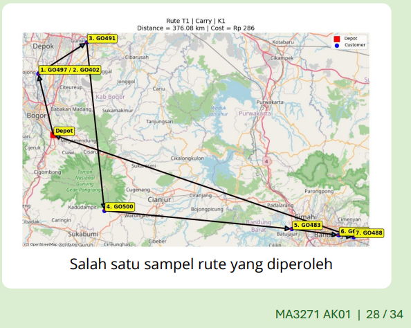
Fun fact: last semester, a student team modeled this same problem — and got results very similar to my first iteration. The routes simply did not make sense to Nutrifood's transporter team.

a sample route from the student model — zigzagging back and forth across West Java

Second Attempt: The Business Changed the Game

1. A big change hit the transporter team: their manager retired. A new "head" came in — with new directions and a new business process that reshaped their working procedures

2. Good news: the delivery date was no longer a decision variable. Why? I was also working on an optimization project with the PPIC team — and one of its outputs is exactly that: the delivery schedule to customers

3. New rule: if possible, all POs from one customer go on one truck

4. Bad news: the computation was still heavy. Removing one variable was not enough

Divide First: Customer Clustering with K-Means

• Main idea: don't optimize 200 customers at once — group them by location first (features: latitude & longitude)
• Honest confession: my first choice was hierarchical clustering with minimum distance (single linkage) as the cluster rule. But after discussing with the team, K-Means was the method they could accept and understand
• Why K-Means won: simple, fast, scales to thousands of customers, easy to explain to the business team
• Number of clusters k chosen with the Elbow Method — plus iterations with the wisdom of the transporter team
• VRP runs per cluster → solutions come out an order of magnitude faster

The critical trade-off: too many clusters → too many sub-problems; too few → each cluster is still too big. This k is the most important hyperparameter of the whole system.

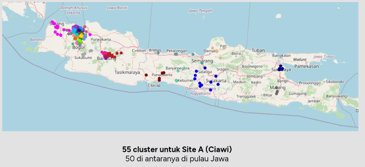
55 clusters for Site A (Ciawi) — 50 of them on Java island

The New Pipeline: Single-Drop vs Multi-Drop

1. Recap all POs per customer → decide who is single-drop (one dedicated truck) and who is multi-drop (shares a route)

2. Single-drop test, against the largest vehicle the customer can accept: total tonnage ≤ truck capacity, total volume ≤ truck capacity, and fill ratio > 80%

3. If a customer's total exceeds the biggest truck → the order is split, and the split itself is optimized with DSO so part of it becomes single-drop

4. Then DSO solves the VRP on the multi-drop orders and the split leftovers — using library(TSP) in R as the tool to evaluate the cost and distance of every agent. Distances are still Euclidean for now; we are considering real road distances from OpenStreetMap

One More Tweak: Squeezing Routes

Going to Production: A Small OS War

The Daily Pipeline

Parameter Sensitivity — in Business Language

Actually… There Are Three Algorithms

The same DSO principle powers three variants in production:

Demo: NUTREX in Action

So… How Optimal Is It, Really?

• The first and second iterations were not instantly optimal — honest truth
• It took a lot of input from the transporter field team, who understand the problem better than any equation
• Patching the algorithm + parameter tuning, again and again — that is why it is still in use today
• First 3 months: monitoring meetings every 2 weeks, comparing algorithm output vs manual schedules on historical data
• The main metric: total cost — manual schedule vs algorithm schedule

Lessons Learned

Conclusions

• Nutrifood's Transporter Problem = a real, multi-layer VRP — done manually for years, with officer wisdom lost at every resignation
• Clustering reduces dimensionality → one big problem becomes many small, solvable problems
• Dynamic Spiral Optimization: a simple metaheuristic — easy to implement, easy to maintain, converges well
• Measurable impact: shorter distances, lower transport costs, schedules in minutes instead of half a day